Extended Quantum Computing Patterns

Function Table

Aliases: –

Tags:

Intent

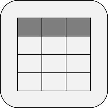
Compute a function table of a finite Boolean function

Context

A classical algorithm must evaluate a given function $f:\{0, 1\}^n \rightarrow \{0, 1\}^m$ for each value of the domain for computing a function table. By exploiting quantum parallelism, a quantum algorithm is able to compute all values of such a finite Boolean function in a single step. This is useful to speed-up algorithms that reveal global properties of a respective function $f$. Note that for $m=1$, a Boolean function $f:\{0, 1\}^n \rightarrow \{0, 1\}$ is often an indicator function which can be used to solve a decision problem.

Solution

For the computation of the function table, the quantum register is split into two parts: The first part consists of $n$ qubits $x$ which represent the domain of the Boolean function $f$ in the computational basis.
The second part of the register contains $m$ qubits $y$ which will be used to represent the values of $f$. The unitary operator implementing the computation of the function table is then defined as:

$$ \newcommand{\colVec}[1]{% inline column vector \bigl( \begin{smallmatrix}#1\end{smallmatrix}\bigr) } \newcommand{\bigColVec}[1]{% inline column vector \left( \begin{matrix}#1\end{matrix}\right) } \newcommand{\state}[1]{{\left| #1 \right>}}U_f \left| x,y\right>=\left| x, y\oplus f(x) \right> $$

As described in Uniform Superposition, the register is first brought in uniform superposition by initializing it as $\newcommand{\state}[1]{{\left| #1 \right>}} \state{0}^{\otimes n} \otimes \left| 0 \right>^{\otimes m}$, and applying the Hadamard transformation $H^{\otimes n}$ on the first part, leaving the second part of the register in the $\newcommand{\state}[1]{{\left| #1 \right>}} \left| 0 \right>^{\otimes m}$ state.
Then, the operator $U_f$ is applied only once to the complete register generating the following function table:

$$ \newcommand{\colVec}[1]{% inline column vector \bigl( \begin{smallmatrix}#1\end{smallmatrix}\bigr) } \newcommand{\bigColVec}[1]{% inline column vector \left( \begin{matrix}#1\end{matrix}\right) } \newcommand{\state}[1]{{\left| #1 \right>}} \state{0}^{\otimes n} \state{0}^{\otimes m} \xrightarrow{H^{\otimes n} \otimes I} \left( \frac{1}{\sqrt{2^n}} \sum_x \state{x} \right) \otimes \state{0}^{\otimes m} $$

$$ \newcommand{\colVec}[1]{% inline column vector \bigl( \begin{smallmatrix}#1\end{smallmatrix}\bigr) } \newcommand{\bigColVec}[1]{% inline column vector \left( \begin{matrix}#1\end{matrix}\right) } \newcommand{\state}[1]{{\left| #1 \right>}}\xrightarrow{U_f} \frac{1}{\sqrt{2^n}} \sum_x \state{x}\state{f(x)} $$

If $f$ is an one-dimensional function (e.g., for solving a decision problem), the register is initialized as $\newcommand{\state}[1]{{\left| #1 \right>}} \state{0}^{\otimes n} \state{1}$.
Afterward, the Hadamard operation is performed on the complete register, i.e. the operator $H^{\otimes n+1}$ is used.
Application of $U_f$ results in the following state:

$$ \newcommand{\colVec}[1]{% inline column vector \bigl( \begin{smallmatrix}#1\end{smallmatrix}\bigr) } \newcommand{\bigColVec}[1]{% inline column vector \left( \begin{matrix}#1\end{matrix}\right) } \newcommand{\state}[1]{{\left| #1 \right>}} \state{0}^{\otimes n} \state{1} \xrightarrow{H^{\otimes n} \otimes H} \left( \frac{1}{\sqrt{2^n}} \sum_x \state{x} \right) \otimes \state{-} $$

$$ \newcommand{\colVec}[1]{% inline column vector \bigl( \begin{smallmatrix}#1\end{smallmatrix}\bigr) } \newcommand{\bigColVec}[1]{% inline column vector \left( \begin{matrix}#1\end{matrix}\right) } \newcommand{\state}[1]{{\left| #1 \right>}}\xrightarrow{U_f} \left( \frac{1}{\sqrt{2^n}} \sum_{x=0}^{2^n-1} (-1)^{f(x)} \state{x} \right) \otimes \state{-} $$

Result

For the general case of $m>1$, the register is in a superposition of all data values in the first register and their corresponding data values in the second register. In the special case of a one-dimensional decision function $f$, the register contains a superposition of all computational bases, where the sign indicates the outcome of the decision function: A minus sign indicates an outcome of 0 whereas a plus sign indicates an outcome of 1 - this is also referred to as "phase kickback".

Related Patterns

This pattern uses Initialization and Uniform Superposition to prepare the initial state of the quantum register. Function tables can be further generalized as Amplitude Amplification. The computation of the function table is done by an Oracle. Often, Uncompute is required to dissolve the created entanglement for subsequent steps of the algorithm.

Known Uses

Many algorithms, including the algorithms of Deutsch, Deutsch-Jozsa, Grover, and Shor make use of function tables.

Deutsch algorithm (PlanQK) Grover's Algorithm (PlanQK) Shor's Algorithm (PlanQK)