Extended Quantum Computing Patterns

"Optimize the parameters of a quantum circuit on a classical computer" (Weigold et al. 2021)

The best solution for a problem must be found or approximated across all possible solutions. An individual solution can be evaluated by an objective function \(C\) that is also given.
By definition, this function is faithful, i.e, its minimum value indicates the best solution (Cerezo et al. 2020). Preferably, \(C\) is also operationally meaningful which means that solutions can be compared: smaller values of \(C\) also indicate better solutions. Since the number of possible solutions increases exponentially with the size of the problems, it is too expensive in terms of computations to evaluate all possible solutions.

–

A hybrid setup is used to evaluate and optimize solutions. On the quantum computer, an initial state is created that may also encode or be varied according to a set of input data \(x\) (refer to the quantum circuit in the upper part of the solution sketch). On this state, an ansatz \(U(\theta)\) is applied which is a circuit that depends on a set of parameters \(\theta\). This results in the \(\newcommand{\state}[1]{{\left| #1 \right>}} \state{\psi_{out}(x,\theta)}\) state. A canonical example of an ansatz is to apply multiple one-qubit operations defining a rotation in the Bloch Sphere around a rotation angle that depends on \(\theta\). However, plenty of other parameterized circuits have been proposed as an ansatz. Then, based on the expectation values of the output state \(\newcommand{\state}[1]{{\left| #1 \right>}} \state{\psi_{out}(x,\theta)}\), the objective function \(C\) for the parameter values \(\theta\) is calculated by the classical computer:

where \(O_i\) is the observable and \(\newcommand{\state}[1]{{\left| #1 \right>}} \left<O_i\right>_{\state{\psi_{out}(x,\theta)}}\) the expectation value of the \(i\)-th measurement to which the function \(f\) assigns an overall cost. If \(C(\theta)\) is sufficiently low, i.e., the termination criteria are fulfilled, the algorithm ends. Otherwise, the parameter set \(\theta\) is optimized further for the next iteration.

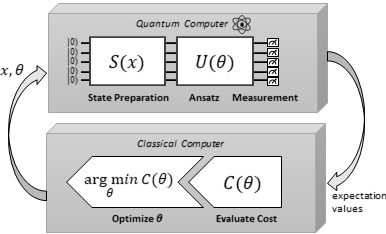
Pattern sketch, taken from: Weigold, Manuela; Barzen, Johanna; Leymann, Frank; and Vietz, Daniel: Patterns For Hybrid Quantum Algorithms. In: Proceedings of the 15th Symposium and Summer School on Service-Oriented Computing (SummerSOC 2021).

However, choosing \(f\), the observables for measuring the qubits and an ansatz is not trivial. The convergence of the algorithm depends on multiple factors: the objective function and the optimization strategy for updating the parameters. Regarding the objective function, one major obstacle for the convergence of the solution are regions of the function which contain only a small norm of the gradient (these regions are also referred to as barren plateaus). These regions can significantly influence how fast the solution converges (Cerezo et al. 2020) or in the worst case, result in non-convergence of the algorithm. Since the optimization procedure is performed classically, the classical computation can impact the overall runtime.

–

This pattern is a refinement of Quantum-Classic Split (Leymann 2019). Within the quantum computation, Initialization (Leymann 2019) is used.

A plethora of algorithms make use of this pattern, e.g., in quantum machine learning this technique was used for developing quantum classifiers (Mitarai et al. 2018), as well as a quantum version of neural networks (Farhi and Neven 2018) or support vector machine (Havlíček et al. 2019), (Schuld and Killoran 2019). A variational algorithm for factorization has been presented in (Anschuetz et al. 2018).

Quantum approximate optimization algorithm (PlanQK) Variational Quantum Eigensolver (PlanQK) Hybrid Transfer Learning (PlanQK) Quantum Boltzmann Machine (Gate-based) (PlanQK)